
VLOOKUP Overview for Excel 2013, Excel 365 and Google Sheets
The VLOOKUP Function is one of the most used, handy, and frustrating functions in Excel. Coincidentally, we receive more inquiries on VLOOKUP uses and issues than most other functions combined. Why is that? First, this function has some strict usage rules in Excel that are not very intuitive. It’s easy to try and use this function without properly setting up your data. As a result, we will cover how to setup VLOOKUP’s properly as well as address common errors. We review how to use VLOOKUP in both Excel and Google Sheets.
At Excelbuddy, our goal was to create one of the most comprehensive overviews for VLOOKUP’s available on the internet.
Comprehensive VLOOKUP Function Glossary
- What is VLOOKUP?
- VLOOKUP Usage Reminders
- Approximate Match vs Exact Match (TRUE vs FALSE)
- First Match
- Multiple Worksheet VLOOKUP
- VLOOKUP Ignores Case Sensitivity
- #N/A Error
- Replace #N/A Errors
- Multiple Criteria Lookup – Index and Match
- VLOOKUP Google Sheets
- Additional VLOOKUP Resources
What is VLOOKUP in Excel?
VLOOKUP is a function in Excel that looks up and retrieves data from a column. Remember that columns are vertical. Thus, we are performing a vertical lookup. This is the opposite of HLOOKUP, where we are performing a horizontal lookup.
For a horizontal lookup in Excel, you would use the HLOOKUP Function.
SYNTAX:
=VLOOKUP (value, table, col_index, [range_lookup])
ARGUMENTS:
- value – Value from first column of a table.
- table – The table from which to obtain a value. We must define this table
- col_index – The column from the table to obtain a value. Cannot be first column.
- range_lookup – TRUE = Approximate Match (default). FALSE = Exact Match.
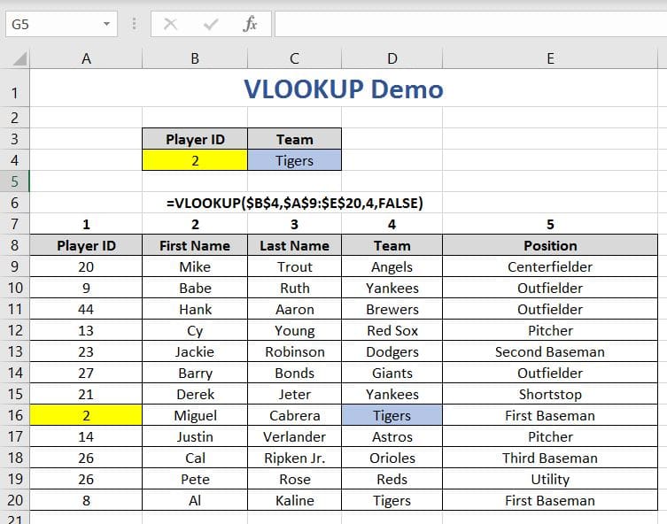
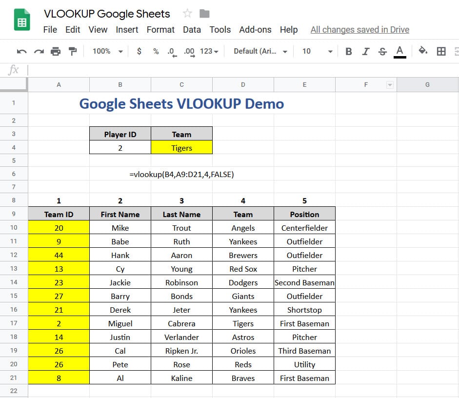
The lookup value, or the value you are matching, must appear in the leftmost column or first column of the table_array . Let’s look at the below example in Fig 1.1. Here the table array starts in column A.
We use this formula: =VLOOKUP($B$4,$A$9:$E$20,4,FALSE)
I always make sure to use absolute cell references, $, when using functions. I find that this helps to prevent broken formulas.
We are telling Excel to look up the value, or Player ID, cell B4. In our example this is 2. This value is then compared to our table which we have identified from A9 – E20. Next, we have Excel return the value if matched from column 4, or D. The columns are numbered A=1 B=2 C=3 etc. We then use FALSE since we would like an exact match.
VLOOKUP Usage Reminders
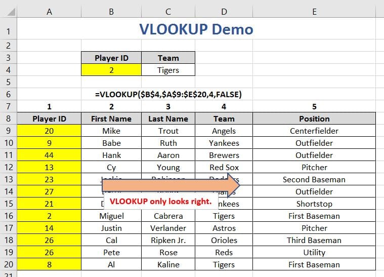
- VLOOKUP Function in Excel only looks to the right. Therefore, once the value is identified from the first column, you can only match from vertical columns to the right.
- Column numbers are sequential alphabetically: A=1 B=2 C=3 etc. Refer to Fig 1.2
- Excel returns the first value that is matched.
- Approximate Match – Excel returns the largest value smaller than the selected value.
TRUE vs FALSE – Approximate vs Exact Match
Approximate Match – Set to True (TRUE)
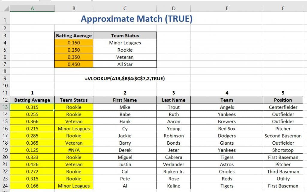
To understand approximate match, we need to understand the word approximate. Approximate is nearly correct, close, but not exact. This is the distinguishing difference between Approximate Match and Exact Match. In the example below, we are using table B4:C4 to return the Team Status of individual players based on their batting averages.
Using the Approximate Match (TRUE) as the range_lookup, Excel compares the batting averages from the lookup table to the value in the selected cell. Let’s look at cell A13. Here, we have a batting average of 0.315. You will notice that we do not have 0.315 in our table. Since we are using an Approximate Match, Excel returns the largest value smaller than our selected value. In our example, that number is .250. Thus, Excel return “Rookie” Refer to Fig 1.5 or download the demo file for a better understanding.
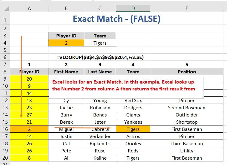
Exact Match – Set to False (FALSE)
By using range_lookup set to FALSE, Excel is told to look for an Exact match (FALSE). This is the most commonly used range_lookup. In the example below, Excel is looking for the Number 2 in column A.
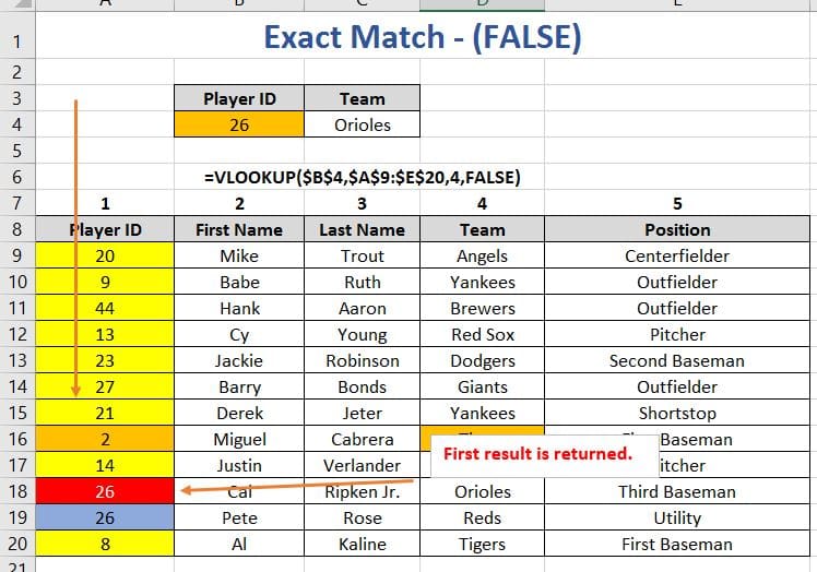
First Match
Please note that Excel will retrieve only the first result. Refer to Fig 1.4 for an example. In this scenario, we we ask Excel to return the Team of the player with ID 26. However, we have two players with the same ID number. Excel solves this problem by only returning the first player, ignoring additional matches.
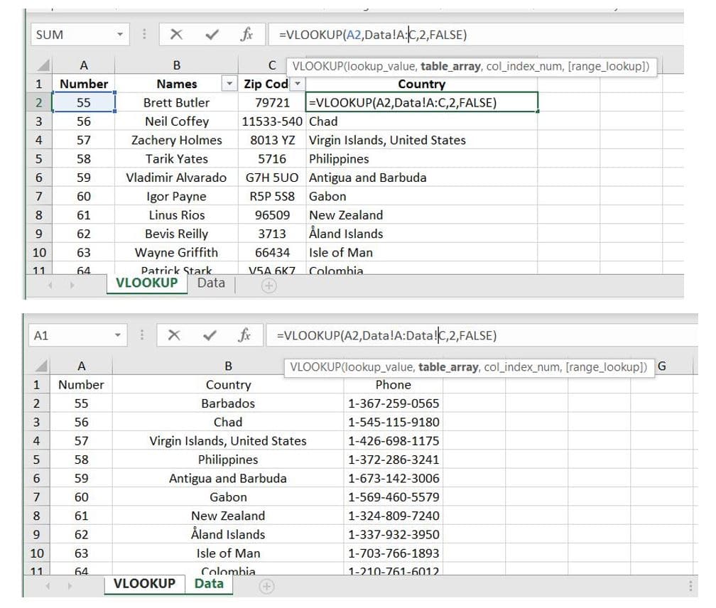
Multiple Worksheet VLOOKUP
Running a VLOOKUP across multiple sheets is very easy. In the example below, you just need to have two of the same identifiers. For example, We are matching the number in column A on both the VLOOKUP worksheet and DATA worksheet. Fig 1.6
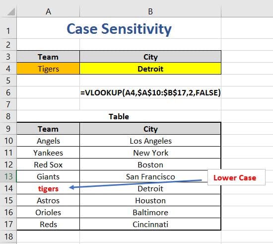
VLOOKUP Ignores Case Sensitivity
The VLOOKUP Function does not care about case sensitivity. Characters can be upper or lower case without impacting the result. Fig 1.7
VLOOKUP Errors
#N/A Error Handling
The dreaded #N/A error. Nothing worse than working on a spreadsheet and getting this error. My curse words have been yelled at computers around the world for this error.
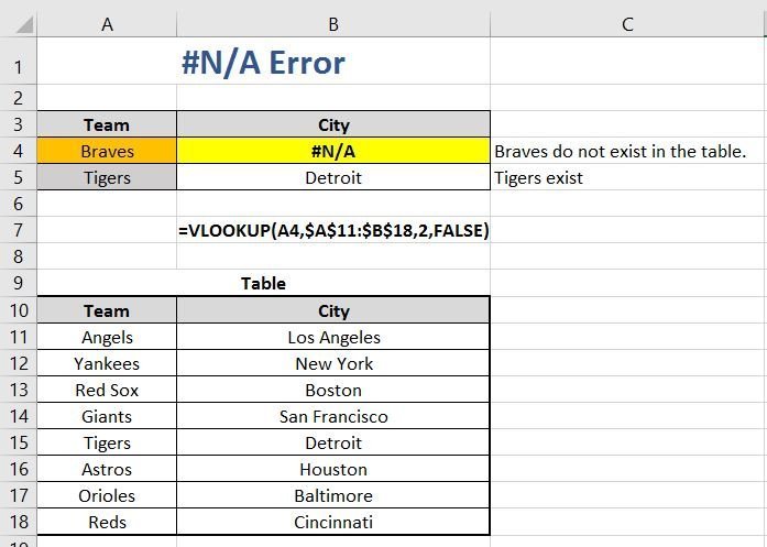
So what is this error? All it means is Excel was unable to find a match.
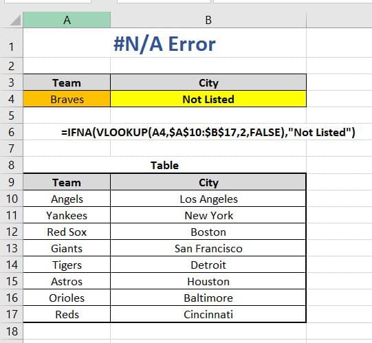
Let’s look at Fig 1.8. In the example below, we are searching for which city the Braves play. As you can see, we do not have a team named the Braves in our tables. As a result, we receive the #N/A Error.
Replace #N/A Errors
Replacing the automated #N/A Error message in Excel is rather easy to do. You can add a default response if Excel is unable to find a match. You can do this by using the IFNA Function.
=IFNA(VLOOKUP(A4,$A$10:$B$17,2,FALSE),"Not Listed")
In this example, we add the IFNA Function to our existing VLOOKUP Function. If a value is not found in out table, we have Excel return “Not Listed.” This will greatly help clean up your spreadsheets.
Multiple Criteria Lookup – Index and Match
VLOOKUP has it’s limitations when trying to perform a multiple criteria lookup. However, there is a relatively easy solution. You can perform a multiple criteria search by using the the INDEX and MATCH function. Check out using the Index and Match Function together.
VLOOKUP Google Sheets
Using VLOOKUP in Google Sheets is very similar to Excel. Unlike Excel, you have to press “F1” to show the formula help screen.
=VLOOKUP(search_key, range, index, [is_sorted])
ARGUMENTS:
- search_key – Value from first column of a table.
- range– The table from which to obtain a value. We must define this table
- index – The column from the table to obtain a value. Cannot be first column.
- range_lookup – (optional) TRUE = Approximate Match FALSE = Exact Match.
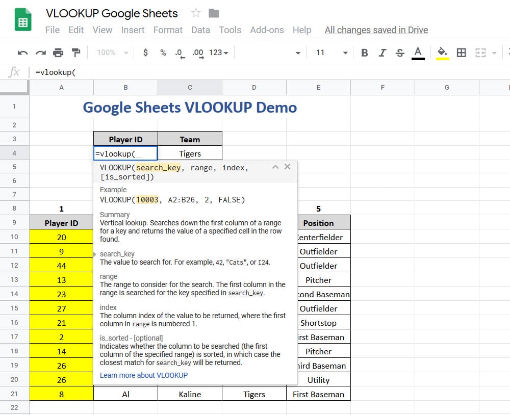
Google Sheets uses difference nomenclatures than Excel, but the basic functionality is very similar. Like Excel, VLOOKUP in Google Sheets searches down the first column then reads to the right.
Additional VLOOKUP Resources
VLOOKUP Function – Fantastic VLOOKUP overview with a plethora of examples. Learn how to use multiple VLOOKUP tables with a nested IF Function.
Pingback: How to use the XLOOKUP Function in Excel - Excelbuddy.com