Overview:
Pivot tables are one of the most versatile and powerful tools available in Excel. They allow you to display data in a table format with multiple filters, and the ability to easily add or remove rows and columns. The first and most important step in creating a pivot table is to set up your raw data in the correct format.
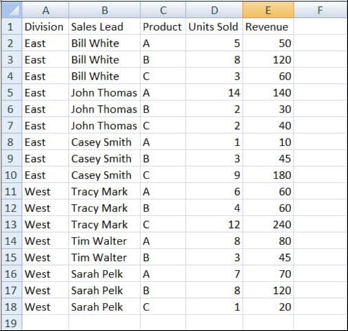
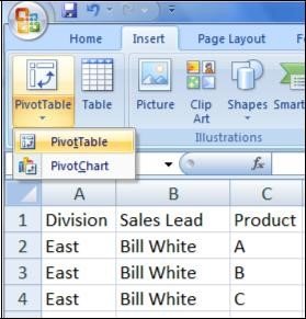
Let’s review setting up data for a pivot table. A name must be present at the top of each column. The header helps to organize the pivot table. In its current format, the information could be useful in telling you that Bill White sold 8 units of Product B and John Thomas had 140 of revenue for Product A. However, what if you wanted to know the total units of Product A sold in the East Division, or the combined revenue of Casey Smith? This would require manually summing the respective values, unless you knew that you could accomplish all of that and more using a pivot table.
Creating a Pivot Table:
To create a pivot table, go to the Insert ribbon and select PivotTable. Please not the option for PivotChart as well. This is basically a pivot table that displays in both a table and chart format. This tutorial covers pivot tables only.
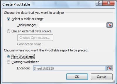
Once you have selected that you want to insert a pivot table, you will be prompted with the Create PivotTable form. We’re using a table/range of data, so the first radio button should be selected.
Enter the range of cells where the data is stored, including the column headings. In this example, that would be cells A1:E18. You then have the option to select where you want the pivot table to be placed. You can select New Worksheet to create the pivot table on a new, separate sheet in the workbook, or select Existing Worksheet and pick a cell in one of the existing sheets to start the pivot table in. Once you’ve designated the data you want to use and where you want the output pivot table to be placed, click OK to create the pivot table.
Pivot Table Field List
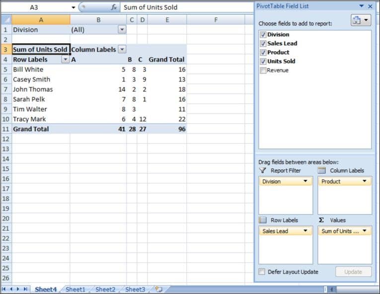
This will open the Pivot Table Field List menu. This shows all of the fields from your dataset which you can arrange as you choose. There are four areas that you can drag the fields to in order to create the pivot table:
- Report Filter: These are overall filters for the entire pivot table. They appear at the top of the table andyou can select one or multiple values from each field. Tables can have multiple filters. In this example, Division was selected as the field to filter the table on.
- Column Labels: Fields dragged into this area will appear as the column headings in the pivot table. You can have multiple fields in this area, and they will appear as tiered headings. In this example, a single heading, Product, was selected as the field for the columns, so the columns show up as A, B, and C. There is also a Grand Total column.
- Row Labels: Similar to column labels, the row labels allow you to select which fields will appear along the rows of the pivot table. Again, you can drag as many fields into the Row Labels area as you would like, and the pivot table will display them in tiers on the rows. In this case, the Sales Lead field was placed in the Row Labels area, so the table shows the names of the six sales leads.
- Values: This area is for the data that will be totaled in the pivot table. In this case, Units Sold was selected for the Values area, so the pivot table displays the total number of units sold. Pivot tables usually default to summing the data, but if you click on the drop down arrow in the Values area, you can click on Value Field Settings to change the Sum function to an Average, Minimum, Maximum, etc. It is possible to show both the Units Sold and the Revenue on the table if you drag both into the Values area.
Aggregated Data
Now that you’ve created the pivot table, you can see how it aggregates the data. It currently shows how many of each product were sold by each sales lead. The vertical and horizontal grand total columns show the total units for each lead and the total number of units of each product sold, respectively.
Filtering Data
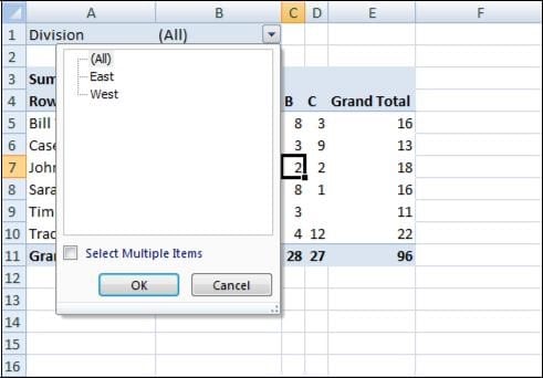
Once you’ve created the pivot table, you have a number of options for filtering the data to modify your views. The most basic way to filter the information is to use the fields that you placed in the Report Filter. In this case, that was the Division field. By clicking the dropdown arrow on the Division filter in the pivot table, you will see your options for filtering. You can select (All), East, or West by clicking on them. If you had a longer list and want to select multiple options, click the Select Multiple Items check box and you will be able to select whichever values from the list you want to include in the pivot table.
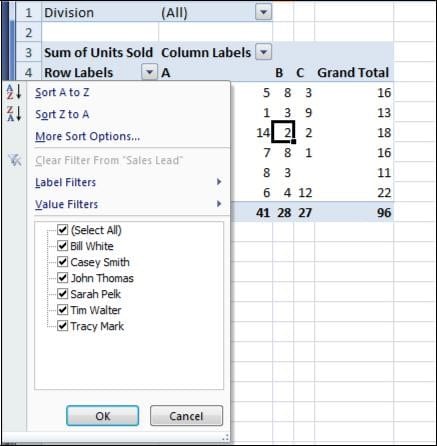
In addition to filtering the entire table using the Report Filters, there are options to filter and sort the columns or the rows. Clicking the dropdown arrow by Row Labels shows the options related to the rows. You can sort the row labels a variety of ways: A to Z, Z to A, or by the values contained in the pivot table (under More Sort Options). The data can be filtered by the labels themselves by selecting Label Filters or by the values in the table by choosing Value Filters. The final way to edit the row labels is to manually pick which labels you want to show using the list of checkboxes. There are similar options if you click the dropdown by Column Labels.
Recap:
This covers the basic functionality of pivot tables, although there are a number of other options to further customize the pivot tables. By right-clicking in the pivot table, you’ll be giving a menu containing a list of the most popular options for pivot tables. You can use this to re-open the Pivot Table Field List menu if you want to go back and drag the fields into different areas to re-arrange the pivot table. There is also an option to Refresh the pivot table if you make a change to the values in your source data.
An even larger list of ways to modify pivot tables can be accessed using the special PivotTable Tools ribbons that appear when you click inside a pivot table. The Options ribbon contains a number of the basic functions including one important one: Change Data Source which allows you to go back to the original pivot table creation form and modify the range of cells on which your pivot table is based. The Design ribbon contains options for changing the format of the table. Pivot tables are immensely customizable and can be tailored to meet most any needs as long as you understand the basics.