
Learn how to use XLOOKUP with multiple criteria in Excel.
In our example, we will show how you can use the XLOOKUP Function with multiple criteria. The functionality is extremely useful and no longer requires multiple functions.
XLOOKUP is also able to handle arrays without having to use special key codes (Ctrl – Shift – Enter). Let’s look at the formula.
In the example below, we will use the criteria located in column I and array data from columns A, B,C, and D. Our result value will be pulled from column E. This follows the standard left to right nature of VLOOKUP.
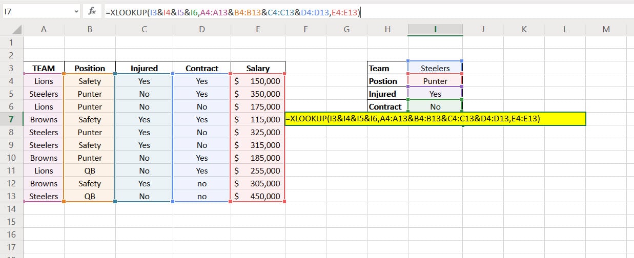
Make sure you pay attention the "&" and "," in the formula.

=XLOOKUP(value1&value2&value3&value4,range1&range2&range3&range4,results_range)

=XLOOKUP(I3&I4&I5&I6,A4:A13&B4:B13&C4:C13&D4:D13,E4:E13)
Let’s look at the first part of the equation:
value1&value2&value3&value4  :  Make you separate with the "&" sign

I3&I4&I5&I6   :   We are selecting our criteria in column I
Next, we need to select the ranges that Excel will be searching through.
range1&range2&range3&range4  :  Again, make sure you use the "&" sign

A4:A13&B4:B13&C4:C13&D4  :  Here we select the columns as shown above.
Finally, we select the range where the result will be selected.
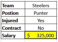
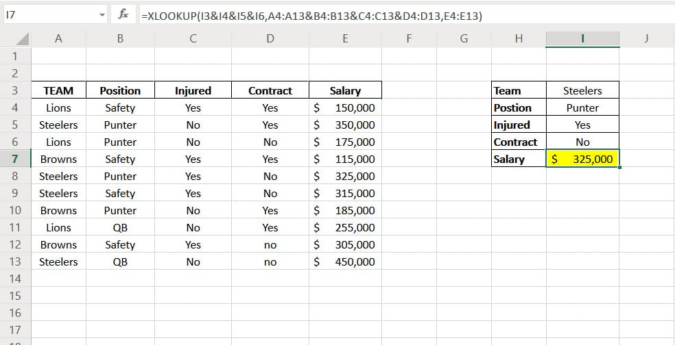
E4:E13 : Excel is grabbing the result of $325,000
This works. Thanks a ton.