Filtering is a fast and easy approach of sorting work with a portion of data so that you are able to display only the rows in your spreadsheet that meets your standard. This can involve rows that have specific numbers or text that are more than or less than a particular number that you have specific about. Filtering will hide these rows that do not meet your criteria temporarily; this put up with you to see only the information that you are interested in. All that you have to do to filter given data is to format the filtering and tag the items that you wish to visualize, everything else will be isolated.
If a spreadsheet is containing a lot of data, it will be difficult to find information fast.
Filters can be used to contract for the information in your spreadsheet, allowing you to be able to view only the information that is relevant to you.
To start Data Filtering:
We need to know how to apply data filtering in Ms-Excel in the example below, we will learn how to apply data filtering in Microsoft Excel.
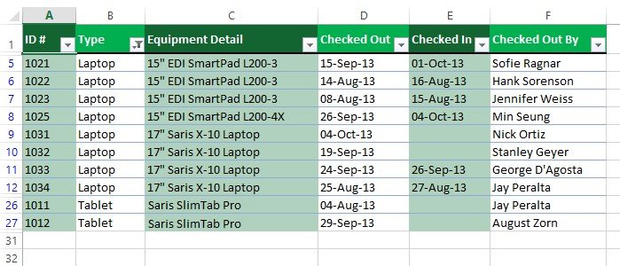
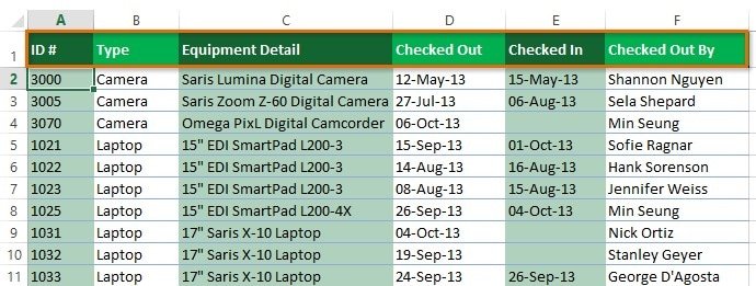
- In order for filtering to work perfectly, your worksheet should have a Header row, which is used to know the title of each column. The worksheet below is arranged into different columns identified by the header cells in row 1
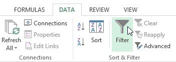
- Choose the data tab, then left click on the filter
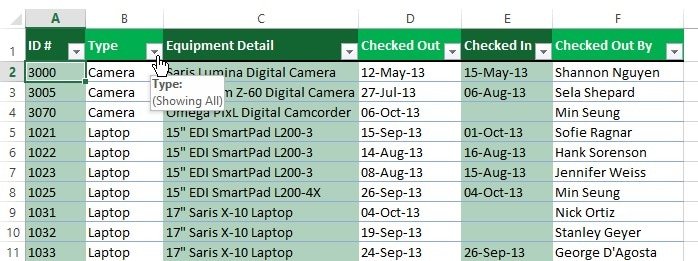
- A pull-down menu will appear in the header cell for each vertical section
- Click the pull-down menu for the column you wish to filter “column B” to view only certain types of equipment.
- The filtering option will appear
- Uncheck the box next to select all to immediately deselect all information
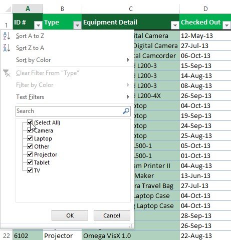
- Check the box next to the data you desire to filter, click ok.
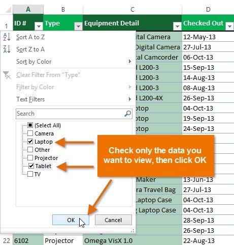
- The information will be filtered, hiding any content that does not fit the criteria.